ARCHIVED: A walkthrough of APackOfTheClones v0.1.x • APackOfTheClones

Introduction

Single-cell RNA sequencing (scRNA-seq) and T cell receptor (TCR) sequencing are popular techniques for studying immune cell function and disease. The combined use of such data can provide insights into clonal expansion. APackOfTheClones provides a simple, publication-ready method to intuitively visualize clonal expansion between different cell clusters with ggplot2, and can be easily slotted into any analysis pipeline.

In this user vignette, we will assume basic familiarity with Seurat and R, and a Seurat object has already been processed through the basic pipeline until at least the UMAP reduction has been obtained. Most importantly, clonal expansion can only be analyzed if the biosample has been run through the 10X genomics Chromium Single Cell Immune Profiling service, and the resulting data processed by Cell Ranger.

We will be showing basic usage of the main function of the package, Namely, in the integration of the 10X genomics T-cell receptor library generated by Cell Ranger into a Seurat object, followed by the usage of a fully customizable clonal expansion plotting method.

Setup the Seurat object and T cell receptor library

Before anything else can be done, we need a Seurat object of the single cell experiment with a dimensional reduction. The most modern and common reduction used in publications is UMAP (Uniform Manifold Approximation and Projection) which is what this package defaults to, and what this vignette will use. There is also a way to base it off of the t-SNE (t-distributed stochastic neighbor embedding) or PCA (Principle Component Analysis) reduction though choosing the latter is probably not the best idea.

library(Seurat)
suppressPackageStartupMessages(library(APackOfTheClones))

# Here, a Seurat object has already been loaded named `pbmc`
print(pbmc)

#> An object of class Seurat 
#> 31053 features across 8000 samples within 1 assay 
#> Active assay: RNA (31053 features, 2000 variable features)
#>  3 layers present: counts, data, scale.data
#>  2 dimensional reductions calculated: pca, umap

Here, we can also see its UMAP reduction plot. It is very important that it is present within the Seurat object so that the later clonal expansion visualization can be based on the coordinates for intuitiveness.

umap_plot <- UMAPPlot(pbmc)
umap_plot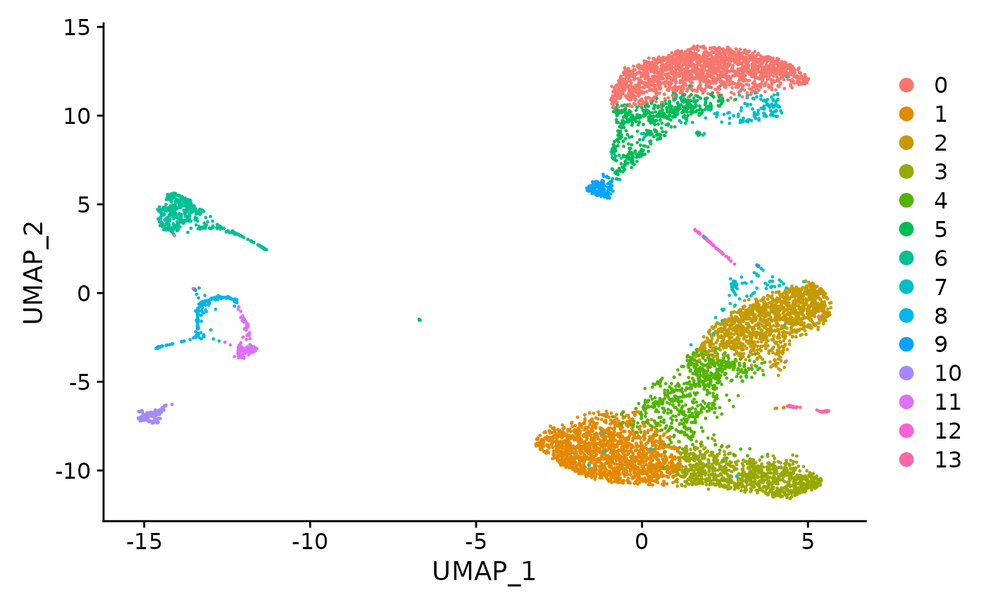

To analyze clonal expansion, the T-cell library (in the form of the all_contig_annotations.csv file) generated by Cell Ranger has to be “integrated” into the seurat object. This simply means that the cell-level receptor information is incorporated into the @meta.data attribute. However, before doing so, let’s quickly view the file structure. An r dataframe of the read-in file has been loaded named tcr_dataframe:

head(tcr_dataframe)

barcode	is_cell	contig_id	high_confidence	length	chain	v_gene	d_gene	j_gene	c_gene	full_length	productive	cdr3	cdr3_nt	reads	umis	raw_clonotype_id	raw_consensus_id
AAACCTGAGTTAACGA-1	True	AAACCTGAGTTAACGA-1_contig_1	True	362	TRB	None	None	TRBJ2-5	TRBC1	False	None	None	None	23679	4	clonotype4	None
AAACCTGAGTTAACGA-1	True	AAACCTGAGTTAACGA-1_contig_2	True	872	TRB	TRBV19	TRBD1	TRBJ1-1	TRBC1	True	True	CASSIRVNTEVFF	TGTGCCAGCAGTATCAGGGTAAACACAGAAGTCTTCTTT	3993	3	clonotype4	clonotype4_consensus_2
AAACCTGAGTTAACGA-1	True	AAACCTGAGTTAACGA-1_contig_3	True	324	Multi	None	None	TRAJ50	TRBC1	False	None	None	None	4870	2	clonotype4	None
AAACCTGAGTTAACGA-1	True	AAACCTGAGTTAACGA-1_contig_6	True	749	TRA	TRAV10D	None	TRAJ49	TRAC	True	True	CAARDTGYQNFYF	TGTGCAGCAAGGGACACGGGTTACCAGAACTTCTATTTT	14844	5	clonotype4	clonotype4_consensus_1
AAACCTGCATCCGGGT-1	True	AAACCTGCATCCGGGT-1_contig_1	True	557	TRA	TRAV19	None	TRAJ56	TRAC	True	True	CAAGGGNNKLTF	TGCGCAGCAGGAGGAGGCAATAATAAGCTGACTTTT	14438	4	clonotype5	clonotype5_consensus_2
AAACCTGCATCCGGGT-1	True	AAACCTGCATCCGGGT-1_contig_2	True	619	TRB	TRBV5	TRBD1	TRBJ1-4	TRBC1	True	True	CASSLTGISNERLFF	TGTGCCAGCAGCCTCACAGGGATTTCCAACGAAAGATTATTTTTC	3721	2	clonotype5	clonotype5_consensus_1

This is the first 5 rows of what the file should look like directly from cell ranger. If you for some reason have some custom version of this dataframe that is different, it is highly important that there AT LEAST exists the column with the column name barcode (column 1) and raw_clonotype_id (column 17), otherwise everything else will not work as intended.

how do I load in the raw file?

library(readr)
tcr_dataframe <- readr::read_csv("your_file_location/all_contig_annotations.csv")

Integration of clonotype information

To finally incorporate the TCR(T-cell receptor library) data into the seurat object, we’ll use the simple integrate_tcr function.

pbmc <- integrate_tcr(pbmc, tcr_dataframe, verbose = FALSE)

Note that the last argument verbose was intentionally set to FALSE due to the presence of a progress bar which corrupts the formatting of the vignette (it defaults to the recommended TRUE). Otherwise, the output to the R Console would have been the following:

#> integrating TCR library into seurat object
#>   |====================================| 100%
#> Percent of unique barcodes: 31 %

By calling integrate_tcr, one can now find all the information from all_contig_annotations.csv within the @meta.data attribute. Let’s take a quick look on what it looks like:

head(pbmc@meta.data)

	orig.ident	nCount_RNA	nFeature_RNA	RNA_snn_res.0.6	seurat_clusters	barcode	is_cell	contig_id	high_confidence	length	chain	v_gene	d_gene	j_gene	c_gene	full_length	productive	cdr3	cdr3_nt	reads	umis	raw_clonotype_id	raw_consensus_id
AAACCTGAGCAACGGT-1	SeuratProject	3456	1203	1	1	NA	NA	NA	NA	NA	NA	NA	NA	NA	NA	NA	NA	NA	NA	NA	NA	NA	NA
AAACCTGAGCAGCCTC-1	SeuratProject	7335	2334	8	8	NA	NA	NA	NA	NA	NA	NA	NA	NA	NA	NA	NA	NA	NA	NA	NA	NA	NA
AAACCTGAGTTAACGA-1	SeuratProject	2949	1144	0	0	AAACCTGAGTTAACGA-1	True	AAACCTGAGTTAACGA-1_contig_1__AAACCTGAGTTAACGA-1_contig_2__AAACCTGAGTTAACGA-1_contig_3__AAACCTGAGTTAACGA-1_contig_6	True	324__362__749__872	Multi__TRA__TRB	None__TRAV10D__TRBV19	None__TRBD1	TRAJ49__TRAJ50__TRBJ1-1__TRBJ2-5	TRAC__TRBC1	False__True	None__True	CAARDTGYQNFYF__CASSIRVNTEVFF__None	None__TGTGCAGCAAGGGACACGGGTTACCAGAACTTCTATTTT__TGTGCCAGCAGTATCAGGGTAAACACAGAAGTCTTCTTT	3993__4870__14844__23679	2__3__4__5	clonotype4	clonotype4_consensus_1__clonotype4_consensus_2__None
AAACCTGCATCCGGGT-1	SeuratProject	3586	1017	0	0	AAACCTGCATCCGGGT-1	True	AAACCTGCATCCGGGT-1_contig_1__AAACCTGCATCCGGGT-1_contig_2	True	557__619	TRA__TRB	TRAV19__TRBV5	None__TRBD1	TRAJ56__TRBJ1-4	TRAC__TRBC1	True	True	CAAGGGNNKLTF__CASSLTGISNERLFF	TGCGCAGCAGGAGGAGGCAATAATAAGCTGACTTTT__TGTGCCAGCAGCCTCACAGGGATTTCCAACGAAAGATTATTTTTC	3721__14438	2__4	clonotype5	clonotype5_consensus_1__clonotype5_consensus_2
AAACCTGCATCTACGA-1	SeuratProject	2659	1141	3	3	NA	NA	NA	NA	NA	NA	NA	NA	NA	NA	NA	NA	NA	NA	NA	NA	NA	NA
AAACCTGGTCTAACGT-1	SeuratProject	5266	1189	0	0	AAACCTGGTCTAACGT-1	True	AAACCTGGTCTAACGT-1_contig_1__AAACCTGGTCTAACGT-1_contig_2	True	565__651	TRA__TRB	TRAV13D-2__TRBV13-3	None__TRBD1	TRAJ38__TRBJ2-7	TRAC__TRBC1	True	True	CAIDPPNVGDNSKLIW__CASSDDRVGEQYF	TGTGCCAGCAGTGACGACAGGGTGGGGGAACAGTACTTC__TGTGCTATAGACCCCCCTAATGTTGGTGACAACAGTAAGCTGATTTGG	7172__13349	2__8	clonotype6	clonotype6_consensus_1__clonotype6_consensus_2

From this snippet of the meta data, we can see that for this particular seurat object, the first 5 columns orig.ident, nCount_RNA, nFeature_RNA, RNA_snn_res.0.6, seurat_clusters were originally present. What we care about is all the new columns after them. A few key things to note: * There are a lot of NA values, and that is due to 1) some cells aren’t T cells, 2) some T cell receptors do not end up being sequenced for many possible reasons, 3) Of the sequenced T cells in the TCR library, there are usually a lot of duplicate barcodes (repeated TCR sequencing of the same cell) as each individual cell may have several TCR types and/or need several contigs to assemble the final sequence. * unique data about TCRs of the same cell (same barcode) are collapsed together with __ in the order of the contigs

Now, the seurat object can be analyzed downstream with the new integrated information however we wish. It also is now ready to have its clonotypes counted and the clonal expansion visualized.

do I HAVE to integrate the the TCR library into my seurat object?

well… no. But there is no reason not to do so and it is heavily recommended to do so. Otherwise, we are about to see in the upcoming clonal expansion plotting function how you can avoid the integration.

How do I get the clonal expansion per cluster information myself?

There is the count_clone_sizes(seurat_obj) function for doing so. Check the documentation by running ?count_clone_sizes for more details.

Ball packing visualization

All one has to do to produce the visualization is by simply running the following code:

pbmc_expansion_plot <- clonal_expansion_plot(pbmc, verbose = FALSE)
# once again, `verbose` is set to false but it defaults to TRUE
pbmc_expansion_plot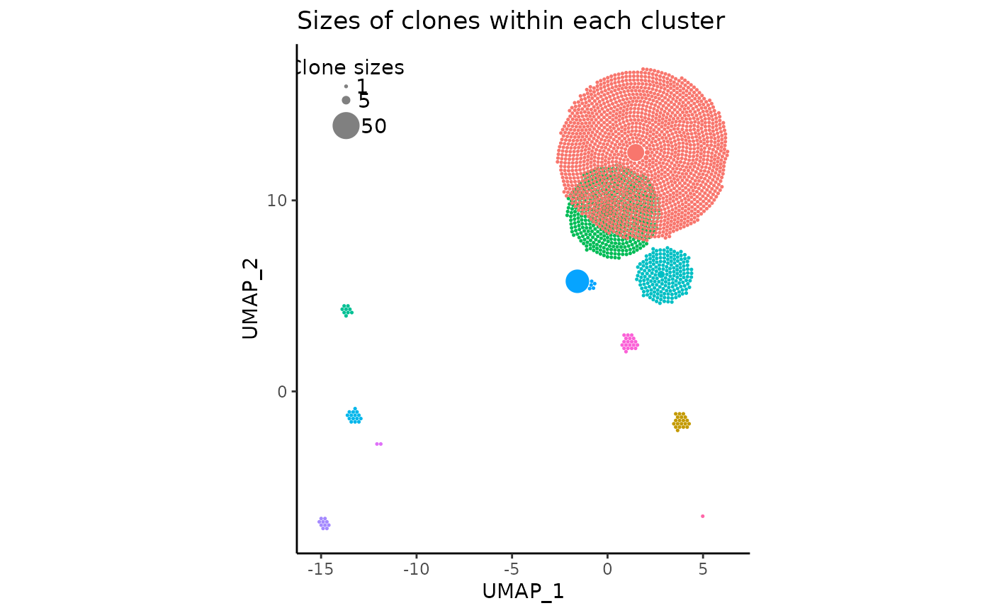

How do I base the clonal expansion plot off of the t-SNE or PCA reduction?

clonal_expansion_plot has an optional argument reduction which defaults to 'umap' that handles which reduction the plot is based off of. The argument can be set to 'tsne' or 'pca' like so:

# t-SNE based plot
pbmc_expansion_plot <- clonal_expansion_plot(pbmc, reduction = 'tsne')
# PCA based plot
pbmc_expansion_plot <- clonal_expansion_plot(pbmc, reduction = 'pca')

A few things to note about the plot

The clonotype counts for each seurat cluster corresponds to their position and color in the original UMAP centroids
The most expanded clonotypes are in the center of each circle cluster with larger sizes, symbolizing increased expansion
There are less circles than the scRNAseq cell count due to aforementioned reasons.
On the top left, there is a somewhat covered visual legend of the relative clone sizes
The red and green clusters have considerable visual overlap
The returned plot is a fully customizable ggplot object

As APackOfTheClones is in a rapid-development phase, the resulting clonal expansion plot will usually not be visually satisfactory on the first run without customizations. However, there are many optional arguments and ggplot tricks that we are about to explore that will help us make it publication quality.

How do I create the plot without integrating the Seurat object and TCR library?

clonal_expansion_plot will also work if the user provides the original seurat object and the raw TCR library dataframe, like so:

# let pbmc be the raw seurat object before the integration
pbmc_expansion_plot <- clonal_expansion_plot(pbmc, tcr_dataframe, verbose = FALSE)

Adjusting intra-cluster spacing

The considerable overlap between clusters (due to the algorithm’s attempt to fit clusters to the original UMAP coordinates) may sometimes obstruct eachother excessively.

To account for this, there are four optional arguments in clonal_expansion plot:

repulse = FALSE,
repulsion_threshold = 1,
repulsion_strength = 1,
max_repulsion_iter = 10

For more details on them, read the “Arguments” section in the function documentation (?clonal_expansion_plot). But to summarize, first, to make the circle clusters move away from eachother, repulse should be set to TRUE, and the function should be ran AGAIN. (If you feel this excessive re-running takes too long or is inefficient for your workflow in its current form, please make an issue on the github page.)

Setting repulse to TRUE with those default parameters should probably yield something like the following:

pbmc_expansion_plot <- clonal_expansion_plot(pbmc, repulse = TRUE, verbose = FALSE)
pbmc_expansion_plot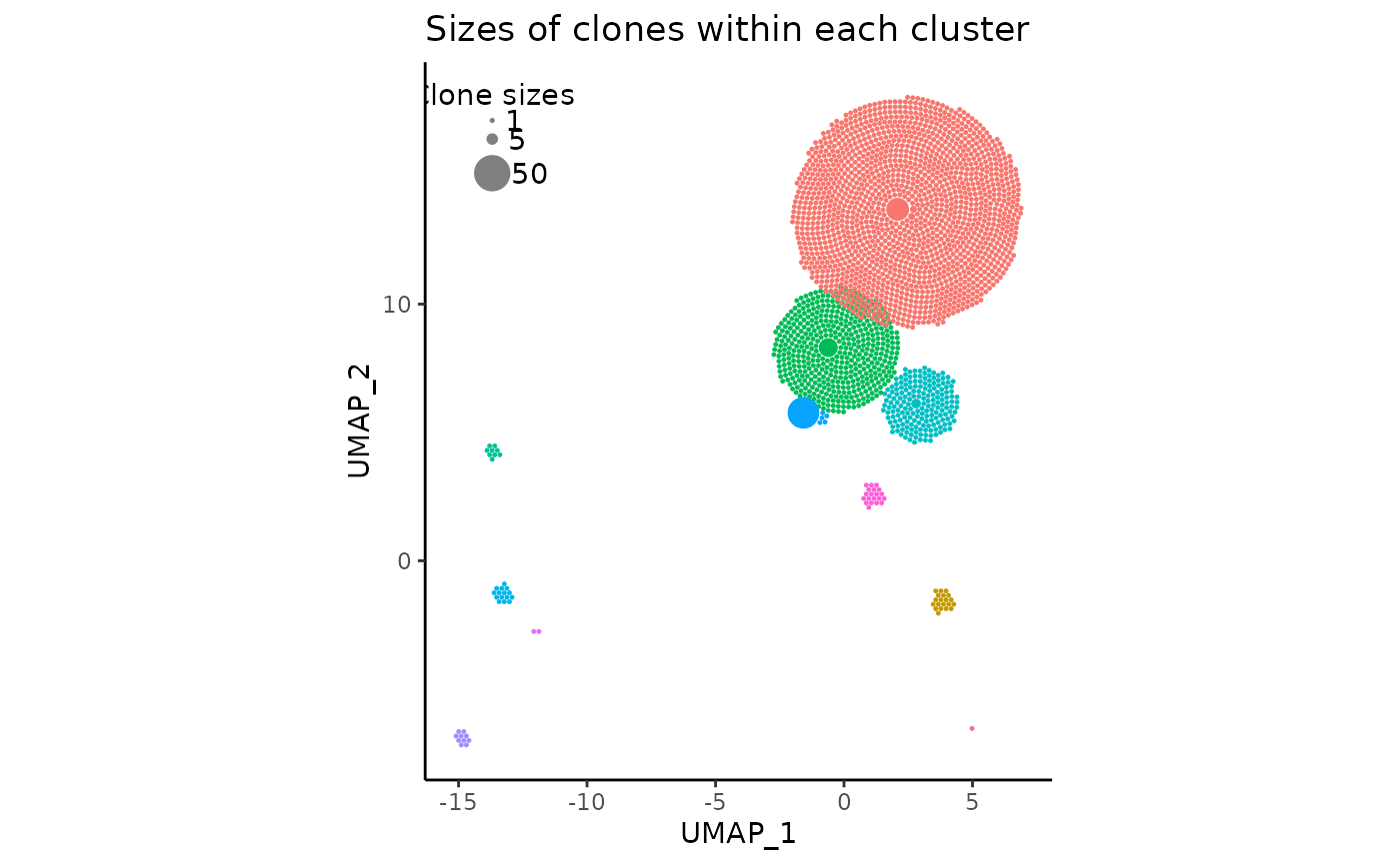

As we can see, the red and green clusters have “moved away” from each other, and there is very little overlap remaining. All other clusters which were not touching remain in their original positions.

Do I HAVE to re-run clonal_expansion_plot each time I want to modify a parameter?

Unfortunately, yes. With the current version (v1) of APackOfTheClones, to change the appearance of the plot, clonal_expansion_plot has to be re-ran with modified parameters each time, which unfortunately may be slow/tedious if a lot of modifications are required. Please create a github issue or contact the author if a new version should be made to prevent this.

If you are still unhappy with the spacing of the plot, see the following ways to adjust the spacing:

repulsion_threshold indicates the amount of ggplot2 units of overlap between clusters that are acceptable. It defaults to 1, meaning that two clusters that overlap by about 1 unit are considered by the repulsion algorithm to not be overlapping. Increasing this number will increase the amount of overlap between clusters, and decreasing this number will do the opposite, while decreasing it to negative values will incur additional spacing between clusters. However, using negative spacing may cause the plot to look very spaced out. Keep reading to see alternatives to doing so.
repulsion_strength relates to how much the clusters should repel each other. The repulsion algorithm works in iterations, where for each iteration, each cluster “pushes” each other away from eachother by some amount. Increasing this value will cause extra “pushing” during each iteration. However, increasing this factor too much may result once again in a very visually unpleasant plot. Note that closer clusters will repell eachother more, and larger clusters will repel smaller clusters more.
max_repulsion_iter indicates the number of iterations where clusters should repel eachother. Increasing this number would ensure that clusters will (almost always) for sure not be overlapping. A trick with this parameter to make more pleasant plots is to decrease repulsion_strength and increase max_repulsion_iter to possibly make a more pleasant arrangement of clusters.

Adjusting and customizing size legend

The plot we’ve generated here has a size legend on the top left, but we see that it is partially outside of the plot. Unfortunately the algorithm for placing the legend is far from perfect in version 0 so the user will have to do a little extra work.

There are the following six parameters to adjust the legend:

add_size_legend = TRUE,
legend_sizes = c(1, 5, 50),
legend_position = "top_left",
legend_buffer = 1.5,
legend_color = "#808080",
legend_spacing = 0.4

Here, we can adjust the argument legend_buffer, which indicates the amount of ggplot2 units to move the legend “inwards” by. We can also slightly increase legend_spacing, an argument specifying the vertical distance between circles in the legend.

# the previous arguments have to be maintained!
pbmc_expansion_plot <- clonal_expansion_plot(
  pbmc,
  legend_buffer = 3,
  legend_spacing = 0.6,
  repulse = TRUE,
  verbose = FALSE
)
pbmc_expansion_plot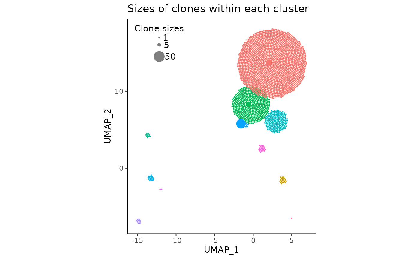

We can even change the circle (clone) sizes displayed in the legend by changing the vector legend_sizes:

pbmc_expansion_plot <- clonal_expansion_plot(
  pbmc,
  legend_sizes = c(1, 5, 25, 50),
  legend_buffer = 3,
  legend_spacing = 0.6,
  repulse = TRUE,
  verbose = FALSE
)
pbmc_expansion_plot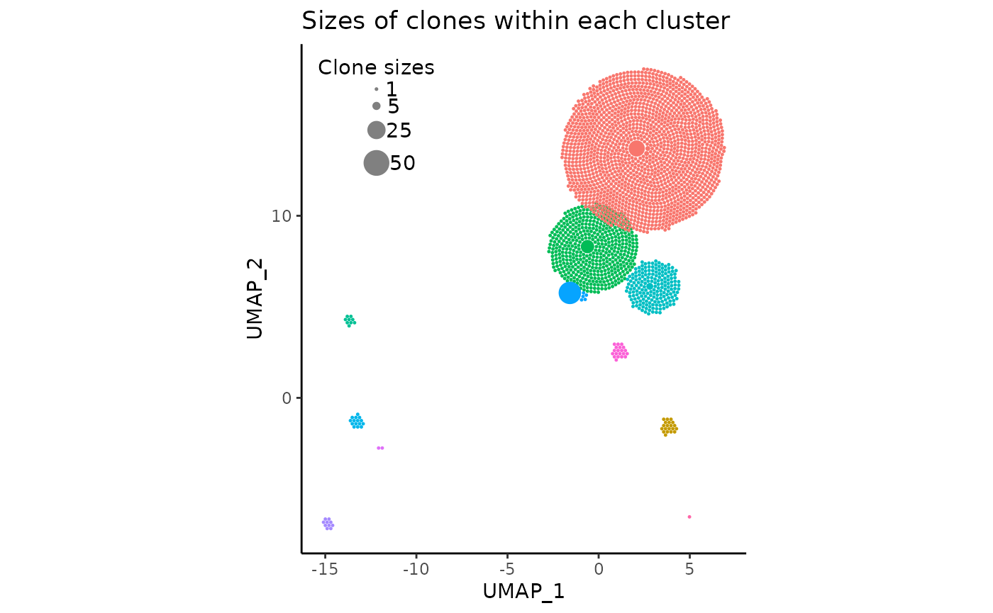

More details about these arguments can be read in the function documentation.

Adjusting and customizing circle size and scaling

So far, the sizes of the individual circles (clones) have seemed to look quite pleasant, fitting roughly into their UMAP cluster centroids snugly. However, this may not always be the case. A likely very common issue upon the initialization of the plot with default arguments is that the circles may be too small or too large.

In these cases, the argument clone_scale_factor should be changed. The argument defaults to 0.1, which is the multiplicative scale factor for the square root radius of a clone. So if a clone size is four, and the factor is 0.1, then the actual radius of the circle on the plot would be sqrt(4) * 0.1 which equates to 0.2.

Additionally, rad_scale_factor can optionally be changed to adjust the intra-circular spacing. The factor defaults to 0.95 and indicates the multiplicative amount to adjust the radius of the circles after they have been placed. decreasing this value (slightly) will basically make each circle smaller in place, increasing the spacing between then,

For demonstration sake, we’ll change the clone_scale_factor to 0.07 and rad_scale_factor to 0.9:

pbmc_expansion_plot <- clonal_expansion_plot(
  pbmc,
  clone_scale_factor = 0.07,
  rad_scale_factor = 0.9,
  legend_sizes = c(1, 5, 25, 50),
  legend_buffer = 3,
  legend_spacing = 0.6,
  repulse = TRUE,
  verbose = FALSE
)
pbmc_expansion_plot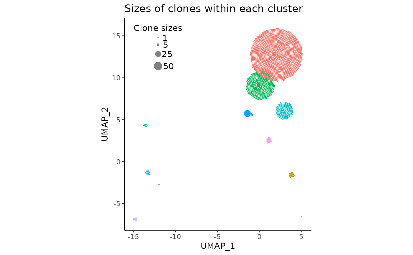

Other possible modifications

There are a few other arguments this vignette did not cover which can be read in the function documentation. However, to end off, one more important argument to consider is use_default_theme = TRUE. It makes the plot have the same axis labels and general theme as the original UMAP plot. If this isn’t to your liking or you want to customize the plot your own way (since clonal_expansion_plot generates a ggplot object!), simply set it to FALSE and you’ll have a very minimally themed plot:

clonal_expansion_plot(
  pbmc,
  use_default_theme = FALSE,
  clone_scale_factor = 0.07,
  rad_scale_factor = 0.9,
  legend_sizes = c(1, 5, 25, 50),
  legend_buffer = 3,
  legend_spacing = 0.6,
  repulse = TRUE,
  verbose = FALSE
)

Additionally, if you really want the plot to reflect the original UMAP plot, you could try using ggplot2’s xlim and ylim functions.

Final product

That’s about it for the most basic functionalities of the clonal expansion visualization function. Remember to save the plot first as an .svg file for maximal resolution, and it should be publication ready.

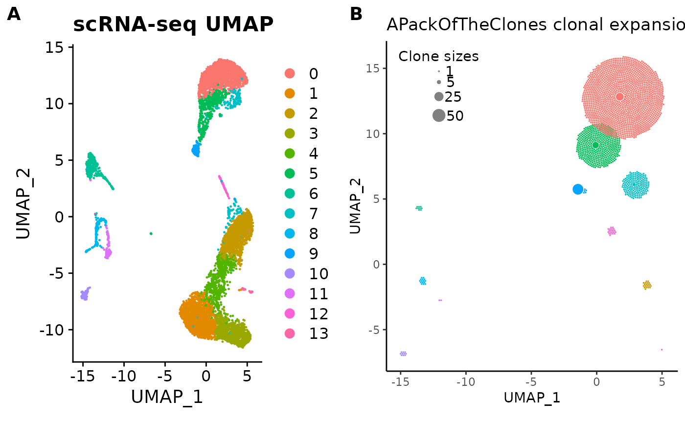
For fun, here’s a side-by-side comparison of the UMAP plot and the clonal expansion plot:

library(ggplot2)
library(cowplot)

cowplot::plot_grid(
  umap_plot + ggtitle("scRNA-seq UMAP"),
  pbmc_expansion_plot + ggtitle("APackOfTheClones clonal expansion plot"),
  labels = "AUTO"
)

How do I reproduce the plots in this vignette?

If you really want to reproduce the plots and code in this vignette, you will need to install the data used in this vignette which has been compiled in an R package SCIPData (Single Cell Immune Profiling Data). You can do so with the following code

# install the data package
library(devtools)
devtools::install_github("Qile0317/SCIPData")

# load the package data directly into R objects in memory
data("pbmc", "tcr_dataframe")

And the rest of the code can be copied and used accordingly.

Alternatively, there are two smaller, minimal, artificial versions of the seurat object and clonotype data that can be loaded in APackOfTheClones, run ?mini_seurat_obj and ?mini_clonotype_data for more details.