Working With Clonotypes Shared Across Clusters

Introduction

A novel feature in this package is the ability to get, filter, and visualize clonotypes that are common across seurat clusters. Potential applications include the ability to quickly and intuitively gauge the rough clonal heterogeneity of certain clusters. Note that in scRepertoire, the scRepertoire::clonalNetwork function does something similar for the original dimensional reductions using arrows, though those display the aggregated degree of commonality between each cluster.

Please read vignette("APackOfTheClones") and ideally also vignette("APackOfTheClones-runs") before reading this vignette. One should then also see that although some of the visualizations in this vignette were produced with the vizAPOTC() function, all visualizations can be replicated with RunAPOTC() and APOTCPlot() that both share parts of the arguments of vizAPOTC().

Getting Clonotypes Common Across Seurat Clusters

getSharedClones() is a convenience function does so while allowing the same seurat object subsetting arguments as seen in vignette("APackOfTheClones"), and returns the clonotypes as a named list where the names are the clonotypes and the elements are numeric vectors where each value is one of the clusters that the clonotype name at its index correspond to.

getSharedClones(
    seurat_obj,
    reduction_base = "umap",
    clonecall = "strict",
    ...,
    extra_filter = NULL,
    alt_ident = NULL,
    run_id = NULL,
    top = NULL,
    top_per_cl = NULL,
    intop = NULL,
    intop_per_cl = NULL,
    publicity = c(2L, Inf)
)

The last five optional arguments allow additional filtering of the shared clonotypes. Most notably, top will filter the resulting shared clonotypes to only those ranked in the top frequencies, either as a proportion or number. More details can be found in the function level documentation for the other arguments. They are especially useful when an experiment has a really high number of single-cells, and the only clonotypes of interest are the most expanded ones.

Here is an example of the function in action, where a combined seurat object is loaded with the variable name pbmc:

head(getSharedClones(pbmc, clonecall = "aa"))
#> $CASLSGSARQLTF_CASSPTVAGEQFF
#> [1] 5 9
#> 
#> $CVVSDFGNEKLTF_CASSLGSGGTGNEQFF
#> [1] 3 5
#> 
#> $CVVSDNTGGFKTIF_CASSVRRERANTGELFF
#> [1] 3 4
#> 
#> $`CAVGEKGYGGSQGNLIF_CASSFRPPGSPLHF;CASHGARGDGFCEKLFF`
#> [1] 3 5
#> 
#> $CARKVRDSSYKLIF_CASSDSGYNEQFF
#> [1] 3 5
#> 
#> $CASLSGSARQLTF_CASSSTVAGEQYF
#> [1] 4 5

Visualizing Shared Clonotypes on an APackOfTheClones Plot

Using the output from getSharedClones(), vizAPOTC() and APOTCPlot() both currently have the exact same arguments to take the information and visually overlay line links between each shared clone. Note that many more changes are to come to this functionality. The arguments are as follows:

show_shared = NULL,
only_link = NULL,
clone_link_width = "auto",
clone_link_color = "black",
clone_link_alpha = 0.5

Where if the output of getSharedClones is inputted into show_shared, the links will be overlaid. The only_link argument will further filter the links so that all links originate from the cluster only_link. The other are aesthetic arguments for the lines and are self explanatory. More details in the function level docs.

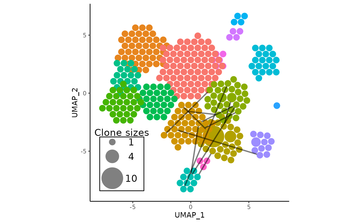
Here is an example, using pbmc:

# get shared amino acid shared clones:
shared_clones_aa <- getSharedClones(pbmc, clonecall = "aa")

# generate the plot
vizAPOTC(
    pbmc,
    clonecall = "aa",
    show_shared = shared_clones_aa,
    verbose = FALSE
)

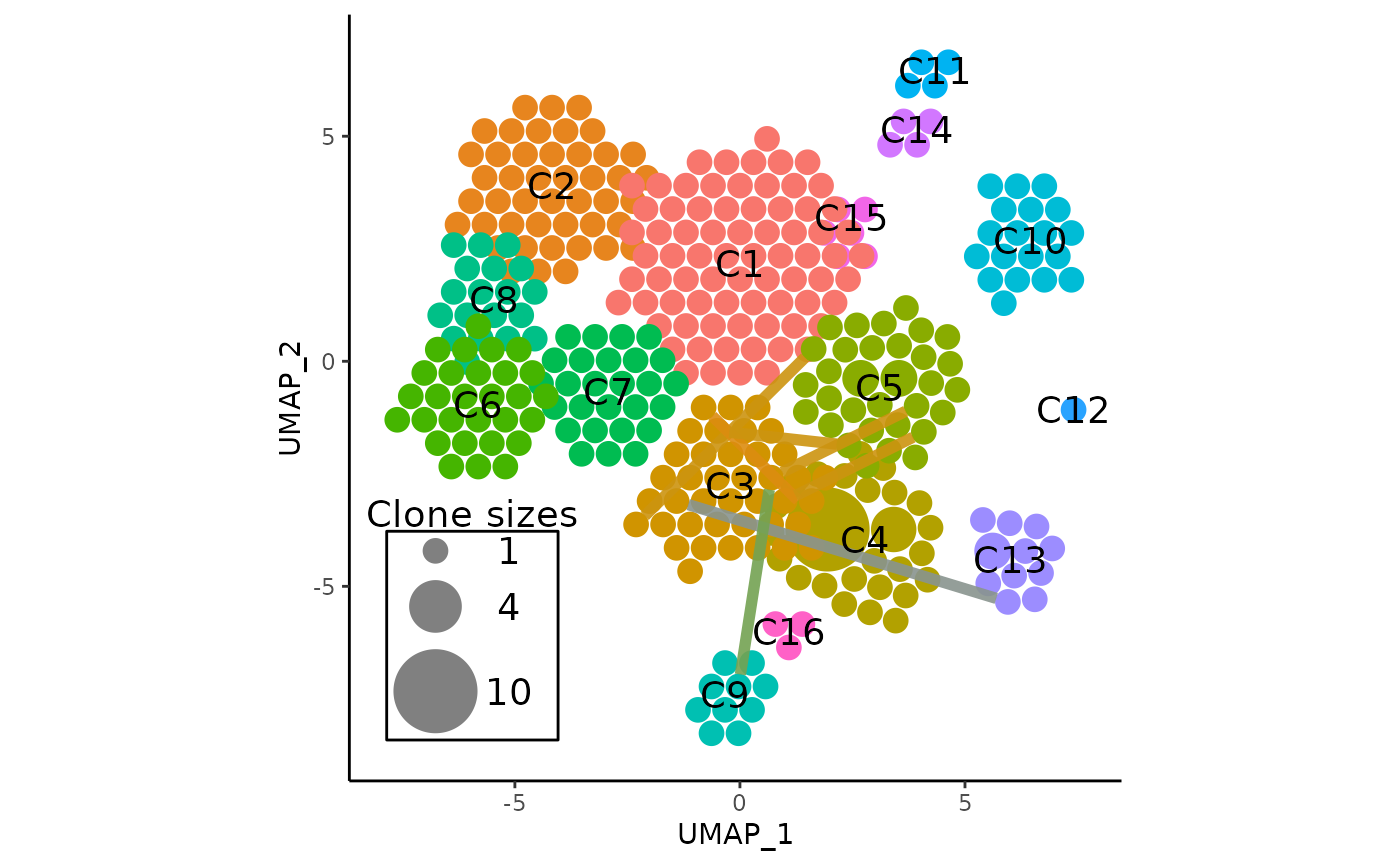
A more useful visualization may be to overlay the links from one cluster, and setting clone_link_color to "blend" which will color each clone link according to the average color of two clusters, for even more intuitiveness:

vizAPOTC(
    pbmc,
    clonecall = "aa",
    show_shared = shared_clones_aa,
    only_link = 3, # only link clonotypes from cluster 3
    clone_link_color = "blend",
    clone_link_width = 2,
    clone_link_alpha = 0.9,
    show_labels = TRUE,
    verbose = FALSE
)

Synergy with showCloneHighlight()

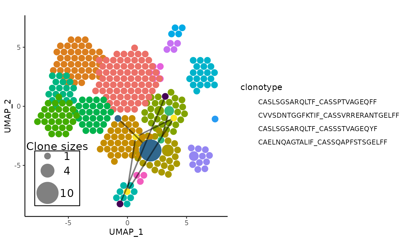
In the interest of inspecting the topmost expanded clonotypes, the topmost clones can be obtained, and the plot of clonal links can have its shared clones highlighted with a different palette than the default ggplot hues, and the non-highlighted sequences can even be slightly dimmed to emphasize the difference. The following is an example of highlighting and linking the top 4 most expanded clonotypes in pbmc:

# For convenience, do an APackOfTheClones Run first
pbmc <- RunAPOTC(pbmc, clonecall = "aa", verbose = FALSE)

# get shared amino acid shared clones for the last run -
# note that the run_id can be replaced with `clonecall = "aa"`
shared_clones_aa_top4 <- getSharedClones(
  pbmc,
  run_id = getLastApotcDataId(pbmc),
  top = 4
)

# generate the unhighlighted plot
linked_apotc_plot <- APOTCPlot(
    pbmc,
    show_shared = shared_clones_aa_top4,
    verbose = FALSE
)

# highlight the top 4 clones with the viridis palette
# also slightly dimming other clones
library(viridis)
showCloneHighlight(
    linked_apotc_plot,
    clonotype = names(shared_clones_aa_top4),
    color_each = viridis(4),
    default_color = NULL,
    scale_bg = 0.95
)

#> * using the latest APackOfTheClones Run Data with object id: umap;CTaa;_;_

Note that to actually get the frequencies of those top clones, one can use the countCloneSizes function.